Controlling a Rigol DS1052E Oscilloscope from Ubuntu Linux


A Rigol DS1052E Oscilloscope. Quite a bargain.


Although I believe it is no longer being made (writing in early 2014), the Rigol DS1052E oscilloscope is still available, and at 250 GBP or less, I think it is amazingly good value for money. If you want a 50MHz digital storage oscilloscope this is a very good way to go IMHO. I bought one in 2012 and it has proved to be very useful. I know some people don't like them, claiming they are inaccurate and poorly built, but I just cannot agree with them. They are neither. To get something significantly better you would need to spend 5 to 10 times as much (last time I looked, anyway).

One of the big advantages of a DSO is that you can control it and read waveforms from it using a computer. In the case of most modern DSO's (including the Rigol) this is done via USB. Once you have waveform data on your computer, you can analyze it (e.g. with FFTs), plot it, etc.

The Rigol ships with some software to do this. However, by all accounts, it isn't the best feature of this system (by a long way), and - of course - it only works on Windows. Since I wanted to use it with Ubuntu Linux some software needed to be written.

First, however, a confusing point should be cleared up. Basic communication between instruments with USB ports and recent versions of Ubuntu (certainly 12.04 LTS) is built in by default. This is handled by USBTMC. It took quite a while for me to realize this and I looked all over the place for obscure and obsolete downloads, none of which are needed. When the oscilloscope is plugged in, it can be accessed via the /dev/usbtmc devices (e.g. /dev/usbtmc0). USBTMC stands for USB Test and Measurement Class and is a more modern equivalent of GPIB. In fact, the commands sent over USBTMC for an instrument may be identical to the ones sent over GPIB for those (few) instruments that support both.

This means that the fundamental issue of just talking to the thing is solved "out of the box" with recent Ubuntu systems. This makes USBTMC significantly easier (and cheaper) for a user than GPIB (see my GPIB page for more information). A non-clone USB/GPIB interface costs more than the entire Rigol scope, in fact!

The rigol_ds1000 and RigolDSWrap Software

The software I wrote for the Rigol DS1052E can be found here. Documentation (generated by Epydoc) can be found here. It should work with other DS1000 series oscilloscopes, and may be at least a useful starting point for dealing with other Rigol scopes. It is pretty minimal, but more or less does the job (at least, the job I wanted doing!).

As with the code I wrote for controlling GPIB instruments, the Rigol software has two parts:
  • A minimal C++ library: rigol_ds1000.cpp. This defines a Rigol_DS1000 C++ class which provides some basic functions, such as sending one or more commands, reading back integer and floating point values and reading back waveforms. This is compiled in to a .so shared object library.
  • A Python wrapper that accesses the C++ library (or, strictly speaking, C wrappers for various C++ class members) via C-types. This defines a RigolDS class which handles interfacing with the oscilloscope, and a small number of functions for plotting data (via Matplotlib) and doing frequency domain analysis of the data.
The Python wrapper - RigolDSWrap.py - is intended to be the user level access to the oscilloscope.

The functionality provided isn't very high level for the most part (although it would be easy to build more sophisticated things on top of what there currently is).

The best way to use this code as it stands is to make settings manually on the oscilloscope front panel to get the desired information displayed in the usual way, then use this software to get the displayed waveform, along with the key vertical and horizontal parameters, in to the computer. This is the normal "use case" when making various, imperfectly planned, measurements on a system.

If the idea to make a large number of identical measurements on many devices under test, the settings on the scope would, of course, need to be set from the program. This is possible with the current code, using the basic commands defined in the Rigol manual and standard Python functions, but the software isn't currently optimized for that. It wouldn't be hard to add anything needed to make life easier, though.

To build the code from its source, just run ./build.sh. After you plug the scope in to your computer, you will need to set read/write permissions on the usbtmc0 device. Use:
sudo chmod a+rw /dev/usbtmc0
to do this. You can then run the test code in RigolDSWrap.py using:
python RigolDSWrap.py
This should capture a signal from channel 1, plot it, do a frequency domain analysis on it, and plot its spectrum.

The test program in RigolDSWrap.py is shown below. Control of scope settings from the program can be carried out with command() calls. The commands that can be sent are documented in the scope's manual. To do the "real work" of capturing a waveform, use the acquire() call. This will return information on what has been captured - but not the captured data itself. Use read_channel() to read acquired waveform data for a channel.


if __name__ == '__main__':
    # Open a connection to the oscilloscope.
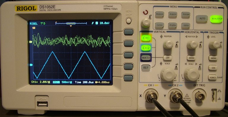
    o = RigolDS()

    # Get the scope's identification string.
    print o.query( '*IDN?' )

    # Set the timebase.
    o.command( ':TIM:SCAL 0.0001' )

    # Acquire the data with the current front panel settings.
    (nch1, nch2, nmax) = o.acquire(1,1)
    print nch1, nch2, nmax

    # If we got channel 1 data, process it.
    if( nch1 > 0 ):

        # Read data and plot it.
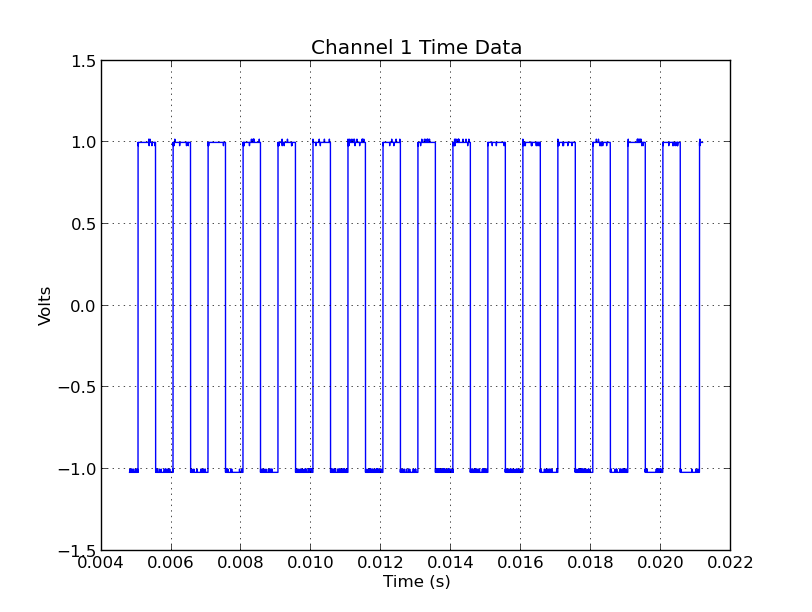
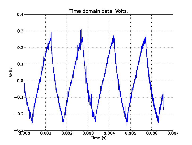
        (nsamples, data, deltat, hoff, voff ) = o.read_channel(1,nch1)
        print "Time domain data. Volts."
        print "samples", nsamples, "time step", deltat, "H offset", hoff, "V offset", voff
        time_plot( nsamples, data, deltat, hoff, 'Channel 1 Time Data' )

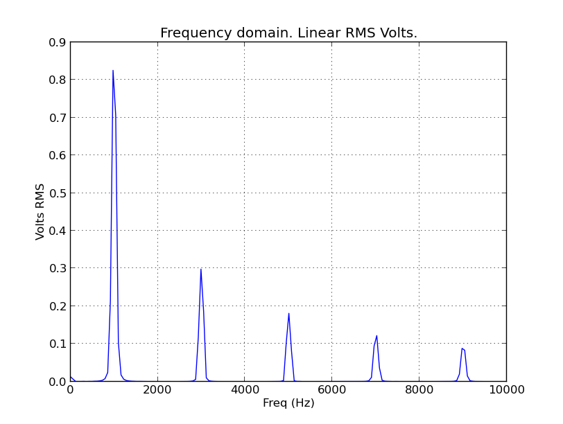
        # Find the amplitude spectrum and plot it.
        print "Frequency domain. Linear RMS Volts."
        ( nfreqs, freq_step, max_freq, spectrum ) = \
            fourier_spectrum( nsamples, data, deltat, False, False, True )
        print "Freq step", freq_step, "Max freq", max_freq, "Freq bins", nfreqs
        freq_plot( nfreqs, spectrum, freq_step, max_freq )

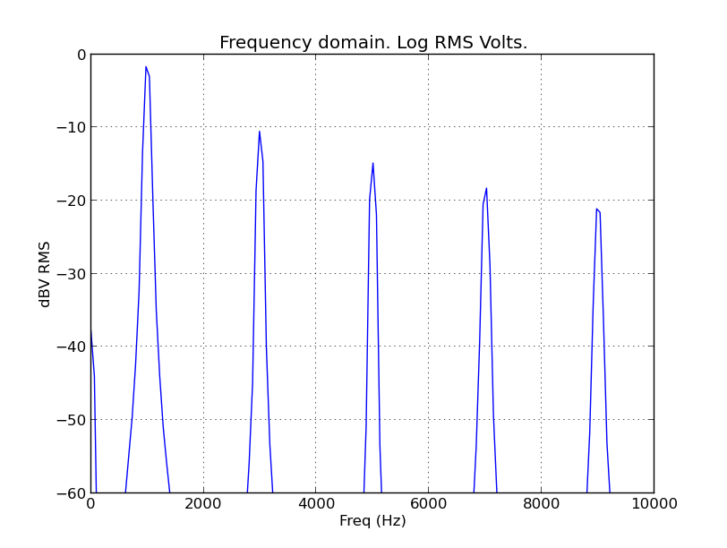
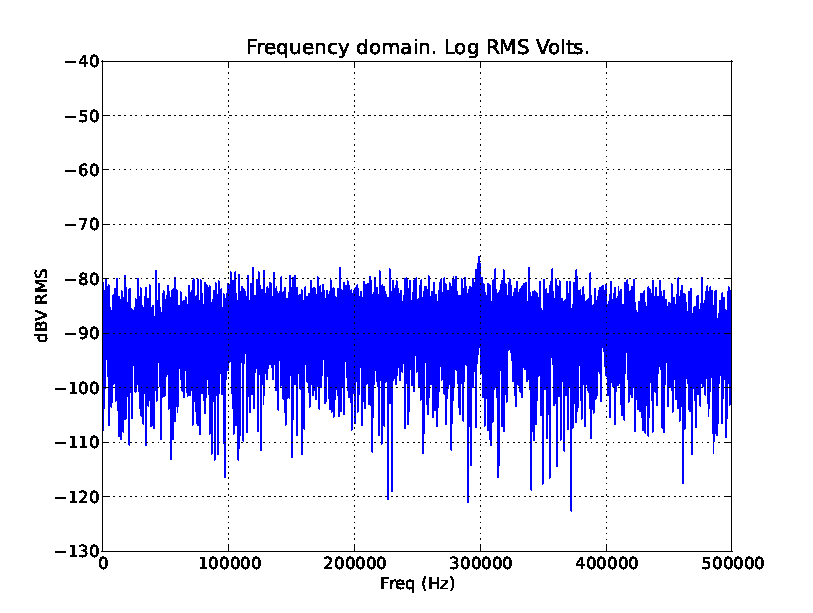
        # Find the log amplitude spectrum and plot it.
        print "Frequency domain. Log RMS Volts."
        ( nfreqs, freq_step, max_freq, spectrum ) = \
            fourier_spectrum( nsamples, data, deltat, True, False, True )
        freq_plot( nfreqs, spectrum, freq_step, max_freq, None, True )

    # Plot channel 2 amplitude vs. time data if we got any.
    if( nch2 > 0 ):
        (nsamples, data, deltat, hoff, voff ) = o.read_channel(2,nch2)
        print nsamples, deltat, hoff, voff
        time_plot( nsamples, data, deltat, hoff, 'Channel 2 Time Data' )


The graphs output from running this program (looking at a 2V peak-peak square wave) are shown below:


The square wave.


The square wave signal in the frequency domain.


The square wave signal in the frequency domain with a log amplitude axis.


Some examples of real measurements made with this software (on a badly misbehaving power supply) are shown below


Noise on the +5V rail shown in the frequency domain. This is OK.


Truly horrible oscillations on the -15V rail.


I hope this software might be of some use to people other than myself. Feel free to do anything you like with it, although I'd be grateful if you acknowledged where it came from if you do use it.


Go home ...